Generating Test Data using Excel: A Sampling Approach using a Data Mart Model

Cetin Karakus
cetin.karakus@gmail.com
version 1.0, Feb 2020 PDF Version

1. Introduction

It is very useful to have access to small, focused datasets during the development and testing of "data-intensive" applications. Though such datasets could be extracted from real data repositories, this is sometimes neither practical nor desirable. For instance, developers might prefer to focus on getting the core algorithms of their application working first  — on a simpler data model — rather than jump into dealing with the messy details of real-world data.

Hand-crafting small datasets for testing purposes is an option but it quickly becomes a time-consuming and soul-destroying laborious task. A completely randomized data generation is another option but ends up producing "alien" datasets that are difficult to relate to and to understand. A better approach is to combine the intuitive curation of hand-crafted datasets with automation and scaling benefits of randomized data generation.

In this paper, we will show a simple, sampling-based test data generation approach using Excel. We found Excel being an excellent environment for test data generation thanks to its very efficient and user-friendly facilities for data entry and manipulation. Moreover, seeing the generated data through an interactive workflow helps with fine-tuning the "hand-crafted" part of the data as needed.

2. Motivating Example: Simple Sales Data Mart

We will explain our data generation approach through a concrete example. To that end, we decided to create a very simple sales data mart example that uses a basic star schema for its data model. We refer to this example as X1.

Data Marts and Star Schema

If you are not familiar with terms like data mart and star schema don’t worry, we will provide some basic explanation of these terms sufficient for following the rest of this paper.

A data mart is a small relational database — often created from data coming from a transactional data source like an order management database — created for efficient data analysis and querying purposes. Its data model is based on a data modeling approach where you have big (i.e. many rows) data tables, called fact tables, that are linked to many satellite tables called dimension tables. Fact tables are linked to dimension tables through foreign keys referencing the records in dimension tables. Whilst fact tables store the actual numeric data that captures an event of interest (e.g. sales, prices, measurements, etc.), dimension tables store "reference data" that embellish/enrich the data captured in the fact tables (e.g. customer to whom sales made to, financial instruments whose price captured, location a given measurement was made at, etc.)

Data marts are stepping stones to bigger databases specifically designed and built for rapid data analysis and reporting purposes called data warehouses. An excellent resource to learn about data warehouses and star schema based data modeling is [DWT03].

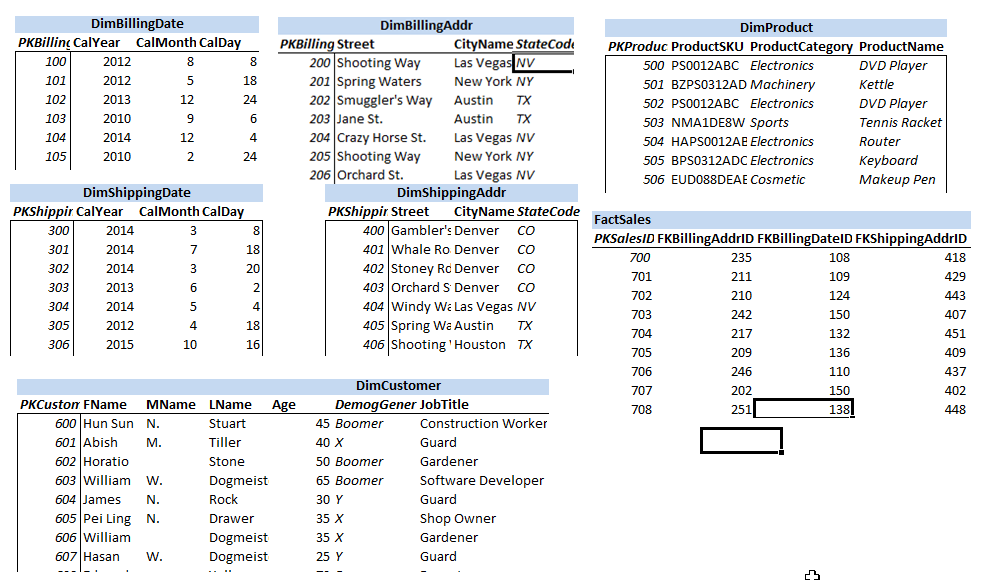
X1 has the following basic star schema:

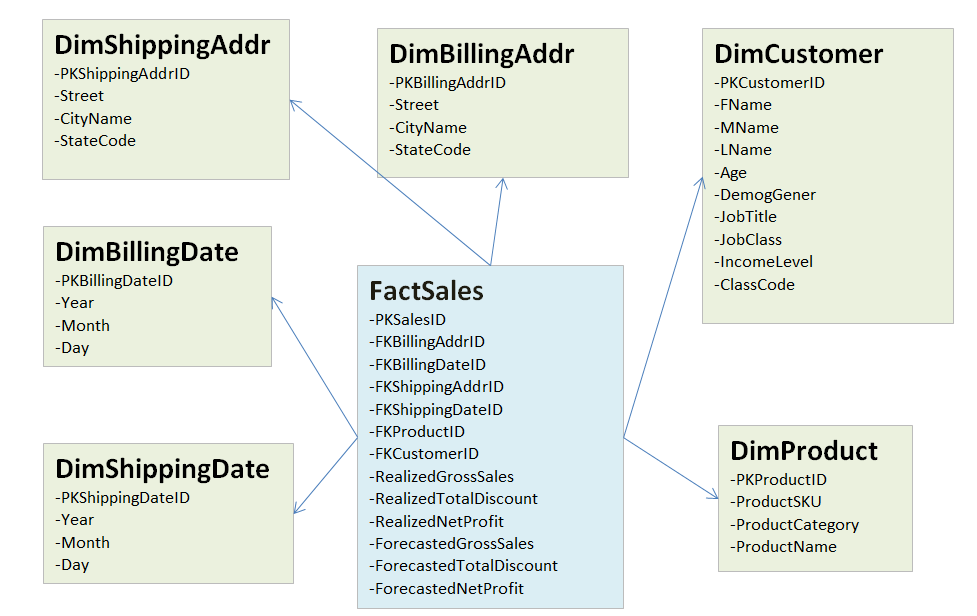
Figure 1. Star schema of X1 sales data mart

Few things come to our attention in the above diagram:

• There are two types of tables in the data model: dimension tables named with "Dim" prefix and fact tables named with "Fact" prefix (There is just one in the example)

• Each table has a primary key named with "PK" prefix and "ID" postfix e.g. PKBillingDateID.

• Fact table FactSales stores the actual data of interest, namely the actual and forecasted sales and discounts

• Dimension tables like DimCustomer, DimProduct, etc. are linked to the fact table FactSales through the foreign keys in the latter (e.g. FKCustomerID, FKProductID).

• Dimension tables store the contextual data that enrich the numerical "event" data stored in the fact table.

• Conceptually same data elements could repeat in different dimension tables. There are two examples of this in the diagram: billing vs shipping address dimensions  — both consisting of the same elements of Street, CityName and StateCode —  and billing vs shipping date dimensions — both consisting of the same date elements — 

Given a data model like the one shown in Star schema of X1 sales data mart, we would like to generate test data that can populate the data tables in the model. Our methodology is composed of several steps:

1. Attribute Consolidation: Create a consolidated list of attributes (elements) making up the data model

2. Attribute Domain Definition: Provide the hand-crafted list of data values that make up the possible values for each attribute

3. Dependent Attribute Resolution: Ensure that attributes which depend on other attributes are consistently defined and used

4. Data Sampling: Sample as many records as needed from the domains of data attributes to create new datasets.

3. Attribute Consolidation

Attribute consolidation step has two major purposes:

1. Create a minimal inventory of data model attributes that will need to be sampled in the data generation process.

2. Conduct basic renaming of data attributes — as necessary and within reasons — to deal with some of the original data model "barnacles"

Consolidated attribute list for X1 data model is shown below:

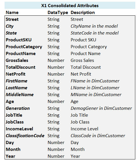
Figure 2. Consolidated list of attributes of X1 model

You will notice that repeating attributes like Street — which occurs both in DimShippingAddr and DimBillingAddr dimensions — are listed only once in the consolidated list. This way, we can define them once — as will be shown in the next section — and use them multiple times.

Some of the attributes in the original star schema model has been renamed in Consolidated list of attributes of X1 model. These are shown in italic in the figure and they have references to the original names in their description columns. The reason we have done this is to show that you have certain possibilities at your disposal at this stage to deal with some of the annoyances of the data model you are dealing with. In our case, we have chosen to use clearer (e.g. instead of FName use FirstName) and more succinct (e.g. instead of StateCode use State) names. We will be using these alternative names in constructing our spreadsheet and settling on "better" names help with making our spreadsheet easier to understand and maintain.

4. Attribute Domain Definition

We define the domain of an attribute as the potential distinct values it can take as far as the data generation process is concerned. We implicitly assume that each value in the domain is equally likely to occur during the sampling process as we do not store any "probability of occurrence" for the values in a domain.

We use a column per attribute to list the potential values an attribute can can take. A partial view of domain definition for X1 is given below:

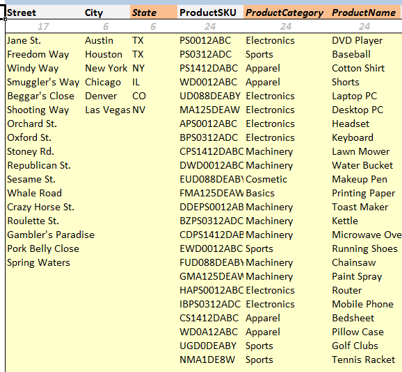
Figure 3. Domain definition for X1 attributes (partial view)

The first line in the figure shows the number of values defined for each attribute (calculated using Excel’s CountA function).

We also define an appropriately named range variable for each attribute (e.g. X1FirstName range for FirstName attribute) in Excel’s name manager — heavily relying on Excel’s Ctrl-Alt-F3 shortcut to define new names quickly — so that we can reference those ranges easily in the data generation process. A partial view of names defined for X1 model are shown below:

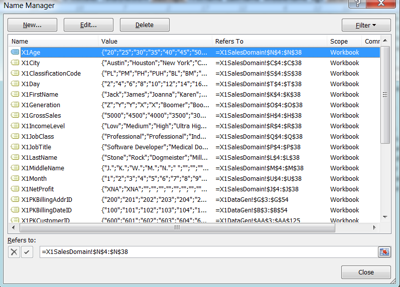
Figure 4. Names defined for X1 attribute values (partial view)

5. Dependent Attribute Resolution

You will notice some color coded attribute headers in Domain definition for X1 attributes (partial view). They refer to what we call dependent attributes: attributes whose value depend on other, independent attributes. For example, given the value of a City, we can determine the value of State that city belongs to. Sampling these two attributes independently will result in data absurdities (e.g. city of "New York" being listed as in the state of "IL"). We avoid this by marking dependent attributes such as State and assigning values to them in a one-to-one correspondence with their independent counterparts.

We will only sample independent attributes in data generation process and simply "look up" the corresponding dependent values. You will see how this is done in Data Sampling section.

6. Data Sampling

Once we have the domains of the all attributes of our data model defined properly, we can proceed with the main activity of actually generating some data.

The main sampling device we use in Excel is RANDBETWEEN() function. It allows to randomly select a value in a number range defined by inclusive lower and upper bounds. We treat that value as a "range index" and select a value from a given Excel range using Excel function INDEX(). As the index value varies randomly, so does the value selected from a target range, allowing us to randomly select values.

For example, suppose we want to randomly sample from the values defined in Excel range "X1TargetRange". The formula we will use will be INDEX(X1TargetRange, RANDBETWEEN(1, CountA(X1TargetRange)),1):

• CountA(X1TargetRange) returns the number of non-empty (i.e. actual) cells in the range. Using CountA() this way gives us the flexibility to define our target ranges big enough to accommodate for future expansion and not to have to adjust range definitions whenever we add a new value to our attribute domains.

• RANDBETWEEN(1, CountA(X1TargetRange)) returns a randomly generated valid index number that can be used to reference a non-empty slot in X1TargetRange range.

• INDEX(X1TargetRange, …​) selects the actual value from the range using the randomly generated index.

6.1. Generating Data for Dimension Tables

We start the implementation of data sampling process from the dimension tables as they are both smaller and simpler to start with and since they are referenced by the fact tables it makes sense to generate values for them first.

You might have noticed that there are primary and foreign keys listed in the original star schema shown in Star schema of X1 sales data mart. Each table in our data model has a unique primary key and such keys are usually auto-generated, sequential numbers which have no particular "business meaning" apart from to uniquely identify records in the data model. As such, it does not make any sense to sample such values. We need to, instead, generate them from a sequence. To that end, using a sequentially increasing list of numbers to assign values to them should be sufficient.

We can always start such sequences from the same fixed value such as "1" but doing so will result in primary keys for different tables being same. This itself is not an issue from a data integrity point of view but causes confusion when looking at the test data where you see the same numbers being used to refer to the records of different tables. We would rather prefer to see different ranges of numbers being used to refer to the records in different tables. To that end, we decided to start the primary keys of different dimension tables for X1 data model from different starting values. You can see this in the following figure:

Figure 5. Using different primary key sequences for X1

We reserve a section of a spreadsheet consisting of several columns for each dimension we want to generate data for. The reserved section will have column headers corresponding to the attributes constituting the dimension in question. Each row in the reserved area corresponds to a record of generated data. Thus, by simply adding more rows we will be able to generate more data.

There are two different mechanisms through which we may generate data for a given attribute:

6.1.1. Sampling

This is used when the attribute is of "independent" type. An example of this is shown below for Year attribute in DimBillingDate dimension:

Figure 6. Sampling for independent attributes

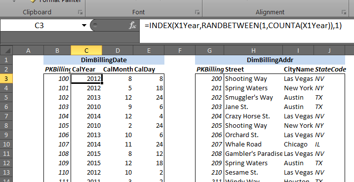
You can see that the formula =INDEX(X1Year,RANDBETWEEN(1,COUNTA(X1Year)),1) is used to sample data. Refer to Sampling Formula Breakdown for a detailed explanation of how such a formula works to generate data.

6.1.2. Lookup

This is used when the attribute is a dependent one. Instead of sampling, we use a lookup based on the already sampled value of the independent attribute on which this attribute depends. An example of this method is shown below for attribute State which depends on the attribute City:

Figure 7. Sampling for dependent attributes

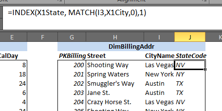
Let’s break down the formula =INDEX(X1State, MATCH(I3,X1City,0),1) that is used:

• Column I stores the values of independent attribute City that is generated through sampling

• MATCH(I3,X1City,0) finds the locational index of the sampled value of City attribute within the list of domain values defined for it

• =INDEX(X1State, …​) looks up the dependent State attribute value in the same row as the sampled independent City attribute value found.

6.2. Generating Data for Fact Table

Fact table FactSales is the central table in the star schema of X1 data model and it references data in the dimension tables such as DimProduct, DimCustomer, DimBillingDate, etc. Moreover, it references those tables through primary keys of the records in those tables. Therefore, we have to have a way to sample primary keys of the dimension tables. We use the same mechanism we used before:

• Define named ranges for the primary keys — which are auto-generated, sequential list of numbers — of each dimension table. For example, we have the named range X1PKProductID for the primary key field PKProductID of the dimension table DimProduct.

• Sample from a primary key range to populate the relevant foreign key field in the fact table. For instance, foreign key field FKProductID of the fact table FactSales uses the sampling formula =INDEX(X1PKProductID,RANDBETWEEN(1,COUNTA(X1PKProductID)),1)

As for the non-referenced fields in a fact table, they fall into two categories:

• First are the those that need to be sampled. These are independent attributes and we sample them as usual. For example, RealizedGrossSales attribute of DimSales is sampled via the formula =INDEX(X1GrossSales,RANDBETWEEN(1,COUNTA(X1GrossSales)),1).

• Rest are the dependent attributes whose values can be computed from sampled values of the independent attributes. For example, RealizedNetProfit is computed as RealizedGrossSales - RealizedTotalDiscount using a simple Excel arithmetic subtraction formula.

The resulting fact table data can be seen below:

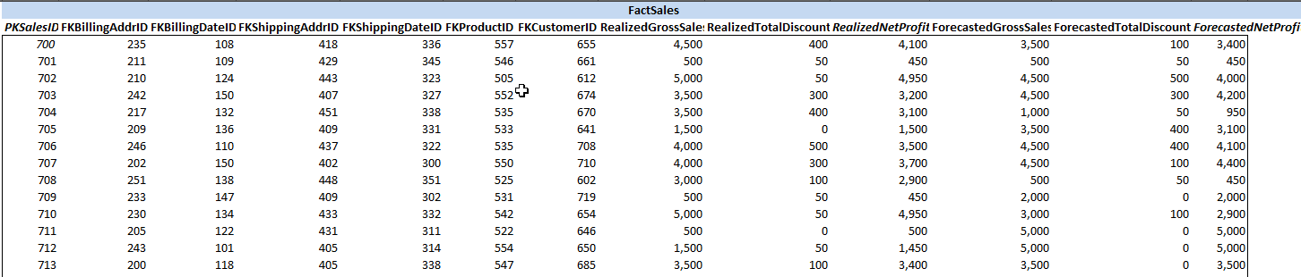
Figure 8. Fact table FactSales data (partial view)

7. Conclusion

Excel can be used to generate test data for relatively complicated data models such as the X1 discussed in this paper. Using the basic sampling approach discussed in the paper results in generating datasets that can be tuned to vary based on the hand-crafted set of data that is used. Excel’s convenient and efficient data entry and manipulation features come very handy in this process and enable generating sufficiently large and varied datasets with relative ease.

The approach we described in this paper is just a basic data generation method and has several shortcomings. Major among them is the inability to deal with joint distribution and corresponding sampling from two or more attributes together. Such a shortcoming has not been a problem for our intended use cases but could be an issue if correlation effects of several attributes occurring simultaneously desired to be modeled.

References

• [DWT03] Ralph Kimball, Margy Ross. The Data Warehouse Toolkit, Third Edition. Wiley. 2013. ISBN: 978-1-118-53080-1

Version 1.0
Last updated 2020-02-23 23:17:04 Central Standard Time